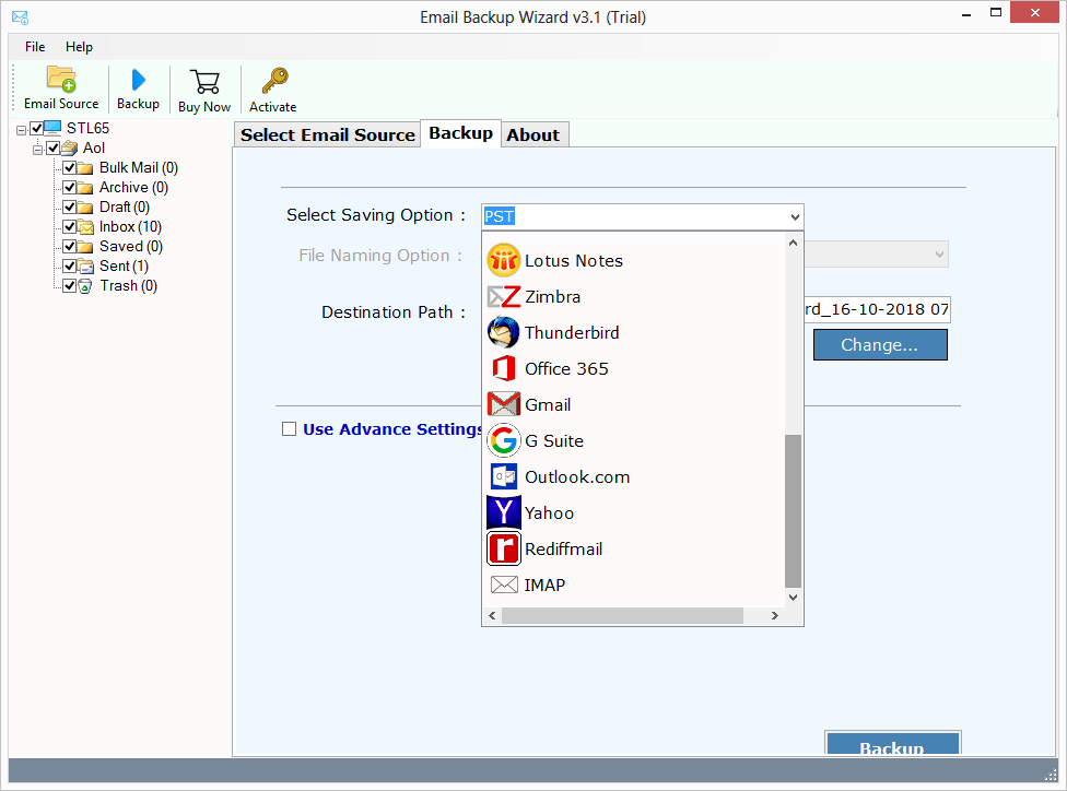
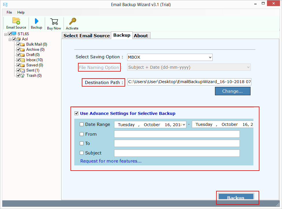
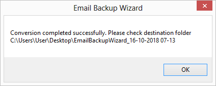
Procedural Screenshots of ZOOK AOL Backup Wizard
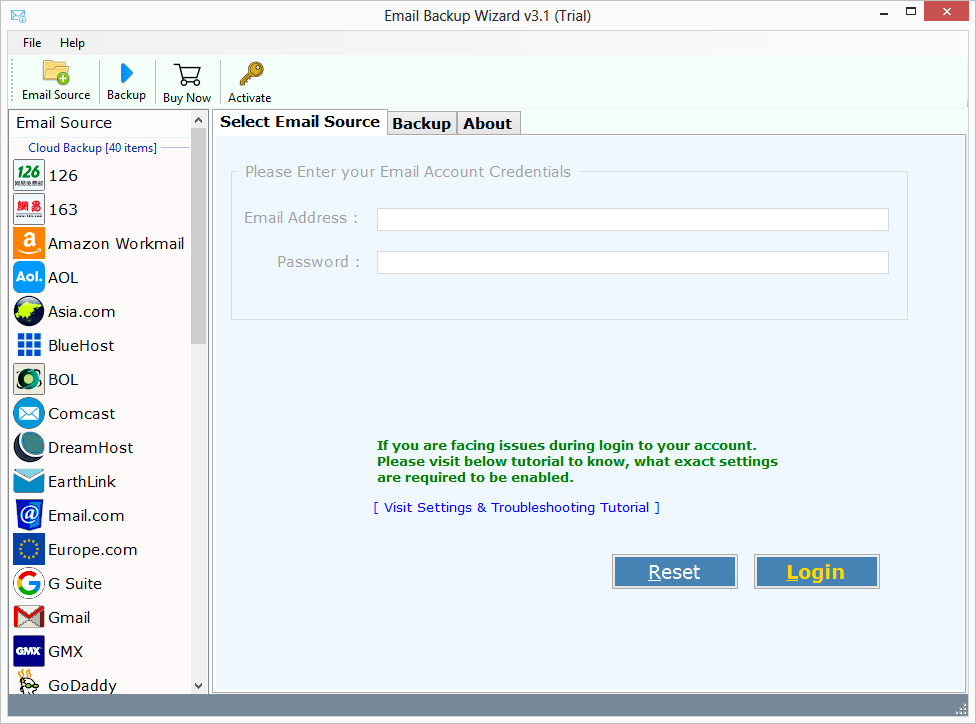
Step 1
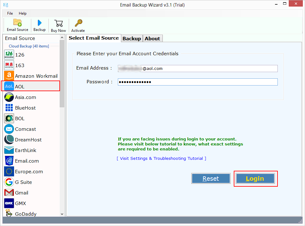
Step 2
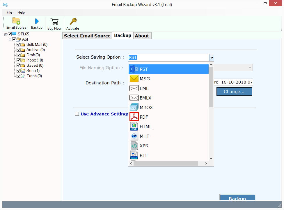
Step 3
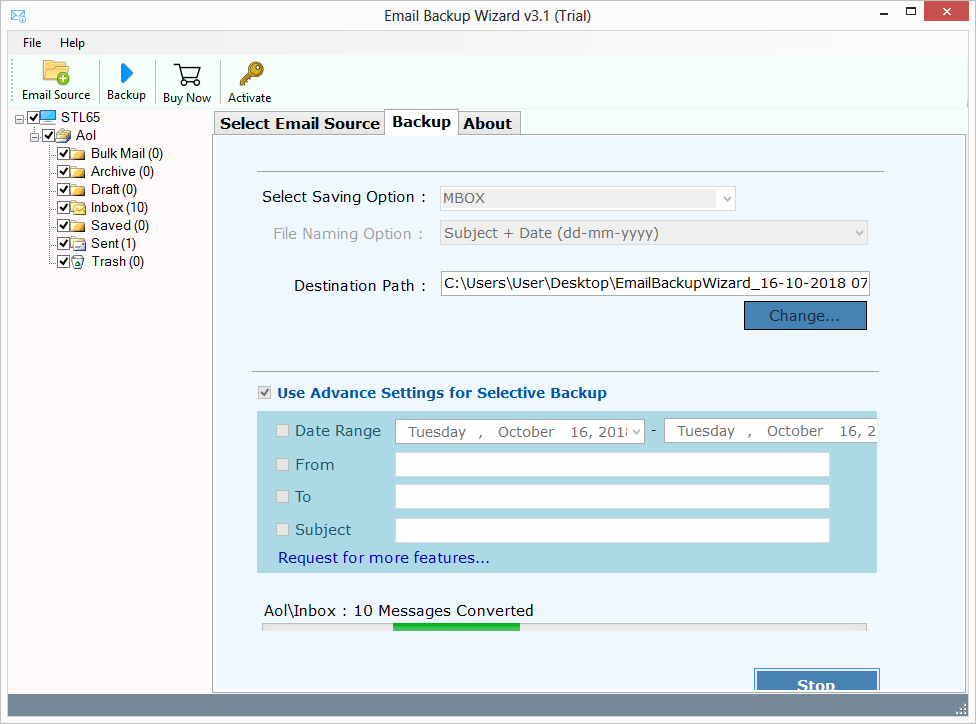
Step 4
: Extension-bending coupling stiffness (zero for symmetric laminates). [D] Matrix : Bending stiffness. First-Order Shear Deformation Theory (FSDT)
Should we add (like clamped edges) using the Ritz method?
% Shear part: 1-point reduced integration (to avoid locking) xi = 0; eta = 0; [N, dN_dxi, detJ] = shape_functions(xy, xi, eta); dN_dx = dN_dxi / detJ; w = 4; % weight for 1-point
% Gaussian quadrature (2x2 points) gauss_points = [-1/sqrt(3), 1/sqrt(3)]; gauss_weights = [1, 1];
This article provides a comprehensive overview of the static analysis of laminated composite plates using First-Order Shear Deformation Theory (FSDT) and provides a functional MATLAB script to calculate deflections. Composite Plate Bending Analysis With MATLAB Code
[NM]=[ABBD][ϵ0κ]the 2 by 1 column matrix; cap N, cap M end-matrix; equals the 2 by 2 matrix; Row 1: cap A, cap B; Row 2: cap B, cap D end-matrix; the 2 by 1 column matrix; epsilon to the 0 power, kappa end-matrix;
We use bilinear shape functions for w and rotations derived from the Kirchhoff constraint. A practical alternative is the discrete Kirchhoff quadrilateral (DKQ) element, but for simplicity we adopt the conforming rectangular element with 12 DOFs.
%% Apply Boundary Conditions fixedDOF = []; for i = 1:nNodes for j = 1:5 if bc_fixed(i,j) fixedDOF = [fixedDOF; (i-1)*5 + j]; end end end freeDOF = setdiff(1:nDof, fixedDOF); Kff = K(freeDOF, freeDOF); Ff = F(freeDOF); Uf = Kff \ Ff;
FSDT, or Mindlin-Reissner plate theory, accounts for transverse shear deformation. It assumes that lines normal to the mid-surface remain straight but not necessarily perpendicular after bending. This theory is required for moderately thick composite plates. Governing Differential Equations
If two opposite edges are simply supported and the other two have arbitrary conditions (clamped, free, etc.), a Levy‑type solution in the form of a single Fourier series in ( x ) and hyperbolic/harmonic functions in ( y ) can be used. This requires solving a characteristic equation for each ( m ). The code can be adapted by replacing the double‑summation with a loop over ( m ) and solving a 4th‑order ODE.
Here ( \barQ_ij^(k) ) are the transformed reduced stiffnesses of the ( k)-th ply.
MATLAB is an ideal tool for this analysis because it handles the matrix inversions and transformations of orthotropic properties seamlessly. This script serves as a foundation; for more complex geometries or boundary conditions, one would transition to the .
%% Visualization figure; surf(X, Y, reshape(w, size(X))); xlabel('x (m)'); ylabel('y (m)'); zlabel('w (m)'); title('Transverse deflection of composite plate'); colorbar; axis equal;
50% Off Reduced Prices!
Standard License
$199$99
Corporate License
$399 $199
Enterprise License
$599 $299
Step 1
Step 2
Step 3
Step 4
Let's Get Started to Resolve Your Problem...
Compatible With
Pre-Requirements
: Extension-bending coupling stiffness (zero for symmetric laminates). [D] Matrix : Bending stiffness. First-Order Shear Deformation Theory (FSDT)
Should we add (like clamped edges) using the Ritz method?
% Shear part: 1-point reduced integration (to avoid locking) xi = 0; eta = 0; [N, dN_dxi, detJ] = shape_functions(xy, xi, eta); dN_dx = dN_dxi / detJ; w = 4; % weight for 1-point
% Gaussian quadrature (2x2 points) gauss_points = [-1/sqrt(3), 1/sqrt(3)]; gauss_weights = [1, 1]; Composite Plate Bending Analysis With Matlab Code
This article provides a comprehensive overview of the static analysis of laminated composite plates using First-Order Shear Deformation Theory (FSDT) and provides a functional MATLAB script to calculate deflections. Composite Plate Bending Analysis With MATLAB Code
[NM]=[ABBD][ϵ0κ]the 2 by 1 column matrix; cap N, cap M end-matrix; equals the 2 by 2 matrix; Row 1: cap A, cap B; Row 2: cap B, cap D end-matrix; the 2 by 1 column matrix; epsilon to the 0 power, kappa end-matrix;
We use bilinear shape functions for w and rotations derived from the Kirchhoff constraint. A practical alternative is the discrete Kirchhoff quadrilateral (DKQ) element, but for simplicity we adopt the conforming rectangular element with 12 DOFs. % Shear part: 1-point reduced integration (to avoid
%% Apply Boundary Conditions fixedDOF = []; for i = 1:nNodes for j = 1:5 if bc_fixed(i,j) fixedDOF = [fixedDOF; (i-1)*5 + j]; end end end freeDOF = setdiff(1:nDof, fixedDOF); Kff = K(freeDOF, freeDOF); Ff = F(freeDOF); Uf = Kff \ Ff;
FSDT, or Mindlin-Reissner plate theory, accounts for transverse shear deformation. It assumes that lines normal to the mid-surface remain straight but not necessarily perpendicular after bending. This theory is required for moderately thick composite plates. Governing Differential Equations
If two opposite edges are simply supported and the other two have arbitrary conditions (clamped, free, etc.), a Levy‑type solution in the form of a single Fourier series in ( x ) and hyperbolic/harmonic functions in ( y ) can be used. This requires solving a characteristic equation for each ( m ). The code can be adapted by replacing the double‑summation with a loop over ( m ) and solving a 4th‑order ODE. %% Apply Boundary Conditions fixedDOF = []; for
Here ( \barQ_ij^(k) ) are the transformed reduced stiffnesses of the ( k)-th ply.
MATLAB is an ideal tool for this analysis because it handles the matrix inversions and transformations of orthotropic properties seamlessly. This script serves as a foundation; for more complex geometries or boundary conditions, one would transition to the .
%% Visualization figure; surf(X, Y, reshape(w, size(X))); xlabel('x (m)'); ylabel('y (m)'); zlabel('w (m)'); title('Transverse deflection of composite plate'); colorbar; axis equal;
What Clients Says

Superb Tool!!! It is all-in-one tool which offers flexibility to download AOL emails in multiple saving options. As I am a user of AOL webmail from the last 6 years. Now I am seeking to import AOL backup to Outlook, then I got this ZOOK AOL backup wizard on Google without losing any data. This tool really works fine for me!!!
A Big Billion Thank you to ZOOK AOL backup software!!! The tool enables us to save AOL webmail to PC of 85 AOL email accounts. It safely takes a backup of AOL emails to flash drive in 25+ file saving formats. Best tool ever with great performance!!!
Hitting Hard by the tool!! The tool has so much interactive interface which enables a safe and secure backup of AOL webmail. It easily saves AOL emails as PDF format with attachments. Apart from it, we are also capable to save AOL as Doc, HML, MBOX, MSG, etc. Wonderful tool!!
Le logiciel de sauvegarde AOL est un excellent outil qui me permet d’exporter des dossiers de messagerie AOL vers un PC local. L'outil dispose de plusieurs options d'enregistrement pour télécharger les dossiers de courrier électronique AOL tels que PST, MBOX, EML, PDF, HTML, etc., et modifier le courrier électronique.